By Andrey Krasovskii, IIASA Ecosystems Services and Management Program
During his workout in the IIASA gym, my colleague Pekka Lauri often runs on a treadmill. He adjusts the velocity of running using the control panel, and it indicates the distance and approximate calories burnt. While Pekka may not be thinking about mathematical models during his workout break, running and other athletic performance can be modeled using some of the same techniques that we use for other questions at IIASA.
Outside of my academic work at IIASA, I am highly interested in sports, and athletics in particular. My wife, Katy Kuntsevich, has won Austrian championships in high jump several times, and my brother, Nikolay, was on his university team as a 400 meter runner.
Visiting my hometown Ekaterinburg, Russia, back in 2014, I got into a dispute with my father, who is a university professor in theoretical mechanics. Namely, my argument was that the sprinters’ acceleration at the finish line of the 100 meter race should be negative. Later on, during the Christmas holidays, I decided to mathematically support my statement.

Left: Prof. Krasovskii with a page from his Lectures in Theoretical Mechanics (Chapter 2, Kinematics, in Russian) featuring Valeriy Borzov on finish. This page was a reason for my study. Top right: Portrait of Isaac Newton.
When athletes run a race, their horizontal velocity can be estimated by modern technologies such as high resolution cameras and lasers. Knowing the horizontal instantaneous velocity, one can calculate acceleration. According to Newton’s law, one can introduce the forces applied to the body center mass of the athlete. Outside a gym treadmill it gets a bit more complicated, with air resistance and headwind or tail-wind. Against these aerodynamic forces the runner applies horizontal force, which drags him forward. In reality it is an “aggregate” of impulsive normal forces generated by feet and the stroke frequency.
The dynamics of an athlete have been described by an ordinary differential equation studied in papers on sprint modeling, first published by physicist J. Keller. This equation has been considered in numerous papers, which have shown that the equation fits the real data for short-distance running (100 and 200 meters). The indicated studies are devoted to the calibration of parameters, to the wind impact analysis, and to the choice of force functions such that the solution satisfies the actual motions, e.g. the running records of Usain Bolt.
The problem of running dynamics reminded me of a type of model that we sometimes use at IIASA, called an optimal control model. Optimal control models are used to calculate the best or most efficient way of doing something, for example, driving from one place to another. If I want to drive from Vienna to Laxenburg, I start my car’s engine at my house (point A). I look at the time, and plan to arrive to IIASA (point B) in 30 minutes. In optimal control terms, the car is a control object, and the driver controls it by pushing the gas/brake pedals and steering the wheel. In the driving process the car meets certain constraints (e.g. the engine power, available roads, and speed limits) and disturbances (e.g. traffic jams, lights, and weather conditions). Obviously, there are many ways of controlling the car in order to reach IIASA in 30 minutes. What if among those admissible controls, I wanted to find an optimal control minimizing car’s energy expenditures during the 30-minute trip from A to B? Here energy is an intensity (cost) of control actions, i.e. fuel (petrol/electricity), or corresponding greenhouse gas emissions. Well, in this case one needs to solve the classical minimum energy control problem. The solution to this problem gives an optimal plan that the car driver (or autopilot) needs to implement. Note, that the corresponding time-optimal control problem consists in finding the fastest driving time to IIASA under given fuel reserve. Optimal control theory (OCT) is an efficient tool for solving such dynamic optimization problems.
My research question was: “Can one control his/her running similar to driving a car?” The answer is: “Yes!”
I applied an optimal control model to Usain Bolt’s performance data at the Beijing Olympic Games in 2008, when he ran the 100 meter sprint in 9.69 seconds. According to the model, under the same conditions he could have distributed his energy optimally and run the distance in 9.56 s. It is worth mentioning that this time is close to his current world record, 9.58 s, achieved at the 2009 World Championships in Berlin. In the paper I also provide modeling results for optimal (energy-efficient) running over 100 m: calculation of the minimum energy and trajectories of acceleration, velocity, and distance from start.
In the conclusion, I argue that applying advanced science in the athletic training programs is far better than doping–better in terms of a healthy body, mind and soul.
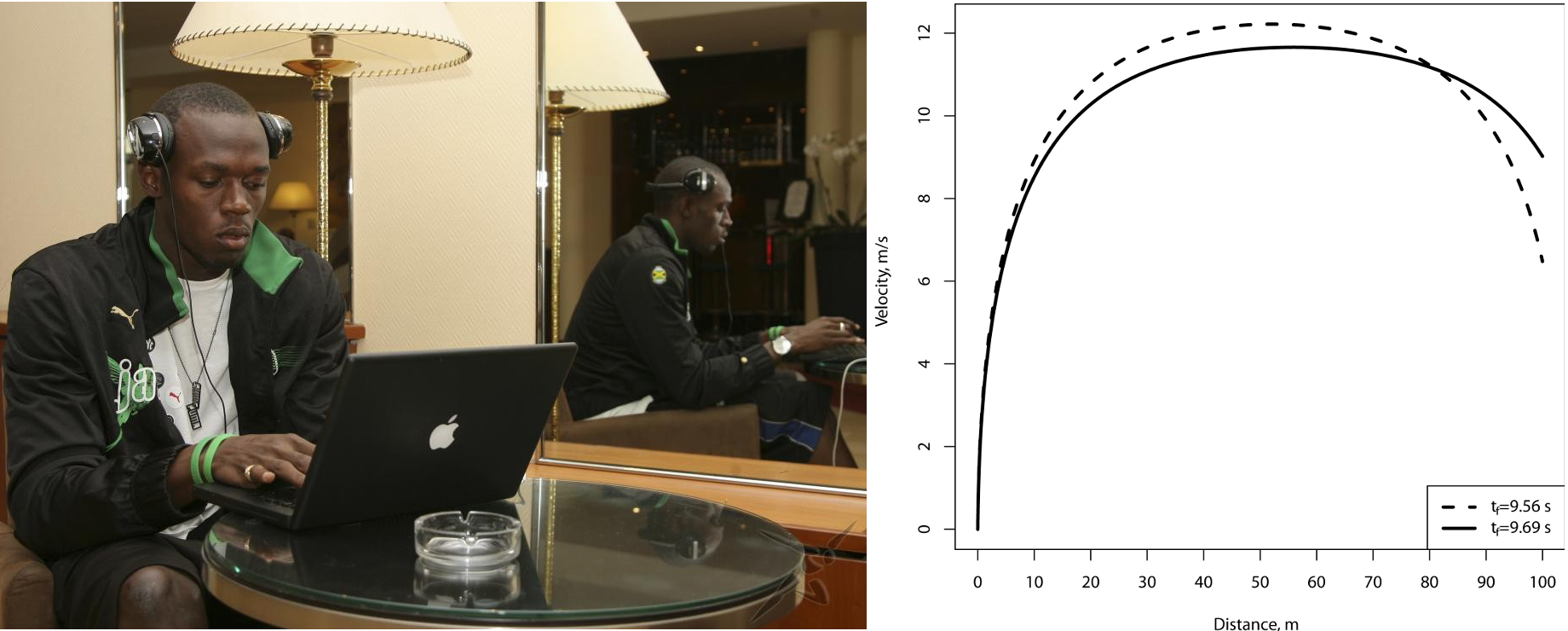
Here is my hypothesis of what Usain Bolt is doing at his laptop. © Weltklasse Zürich – Marcel Giger
Reference:
A. A. Krasovskii, “Application of optimal control to a biomechanics model”, Proceedings of the Steklov Institute of Mathematics, 2015, Vol. 291, pp. 118–126. http://dx.doi.org/10.1134/S0081543815080118
I would like to thank Sergey Aseev, Katherine Leitzell, as well as my colleagues in the IIASA Ecosystem Services and Management Program (ESM) for their interest and valuable discussions.
Note: This article gives the views of the author, and not the position of the Nexus blog, nor of the International Institute for Applied Systems Analysis.
You must be logged in to post a comment.