Jul 26, 2017 | Alumni, Climate Change, Poverty & Equity, Sustainable Development, Water, Young Scientists
Adil Najam is the inaugural dean of the Pardee School of Global Studies at Boston University and former vice chancellor of Lahore University of Management Sciences, Pakistan. He talks to Science Communication Fellow Parul Tewari about his time as a participant of the IIASA Young Scientists Summer Program (YSSP) and the global challenge of adaptation to climate change.
How has your experience as a YSSP fellow at IIASA impacted your career?
The most important thing my YSSP experience gave me was a real and deep appreciation for interdisciplinarity. The realization that the great challenges of our time lie at the intersection of multiple disciplines. And without a real respect for multiple disciplines we will simply not be able to act effectively on them.
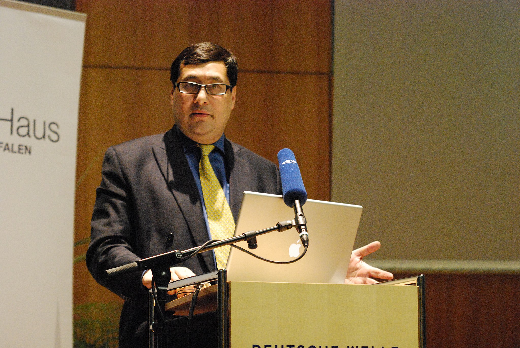
Prof. Adil Najam speaking at the Deutsche Welle Building in Bonn, Germany in 2010 © Erich Habich I en.wikipedia
Recently at the 40th anniversary of the YSSP program you spoke about ‘The age of adaptation’. Globally there is still a lot more focus on mitigation. Why is this?
Living in the “Age of Adaption” does not mean that mitigation is no longer important. It is as, and more, important than ever. But now, we also have to contend with adaptation. Adaptation, after all, is the failure of mitigation. We got to the age of adaptation because we failed to mitigate enough or in time. The less we mitigate now and in the future, the more we will have to adapt, possibly at levels where adaptation may no longer even be possible. Adaption is nearly always more difficult than mitigation; and will ultimately be far more expensive. And at some level it could become impossible.
How do you think can adaptation be brought into the mainstream in environmental/climate change discourse?
Climate discussions are primarily held in the language of carbon. However, adaptation requires us to think outside “carbon management.” The “currency” of adaptation is multivaried: its disease, its poverty, its food, its ecosystems, and maybe most importantly, its water. In fact, I have argued that water is to adaptation, what carbon is to mitigation.
To honestly think about adaptation we will have to confront the fact that adaptation is fundamentally about development. This is unfamiliar—and sometimes uncomfortable—territory for many climate analysts. I do not believe that there is any way that we can honestly deal with the issue of climate adaptation without putting development, especially including issues of climate justice, squarely at the center of the climate debate.
COP 22 (Conference of Parties) was termed as the “COP of Action” where “financing” was one of the critical aspects of both mitigation and adaptation. However, there has not been much progress. Why is this?
Unfortunately, the climate negotiation exercise has become routine. While there are occasional moments of excitement, such as at Paris, the general negotiation process has become entirely predictable, even boring. We come together every year to repeat the same arguments to the same people and then arrive at the same conclusions. We make the same promises each year, knowing that we have little or no intention of keeping them. Maybe I am being too cynical. But I am convinced that if there is to be any ‘action,’ it will come from outside the COPs. From citizen action. From business innovation. From municipalities. And most importantly from future generations who are now condemned to live with the consequences of our decision not to act in time.
© Piyaset I Shutterstock
What is your greatest fear for our planet, in the near future, if we remain as indecisive in the climate negotiations as we are today?
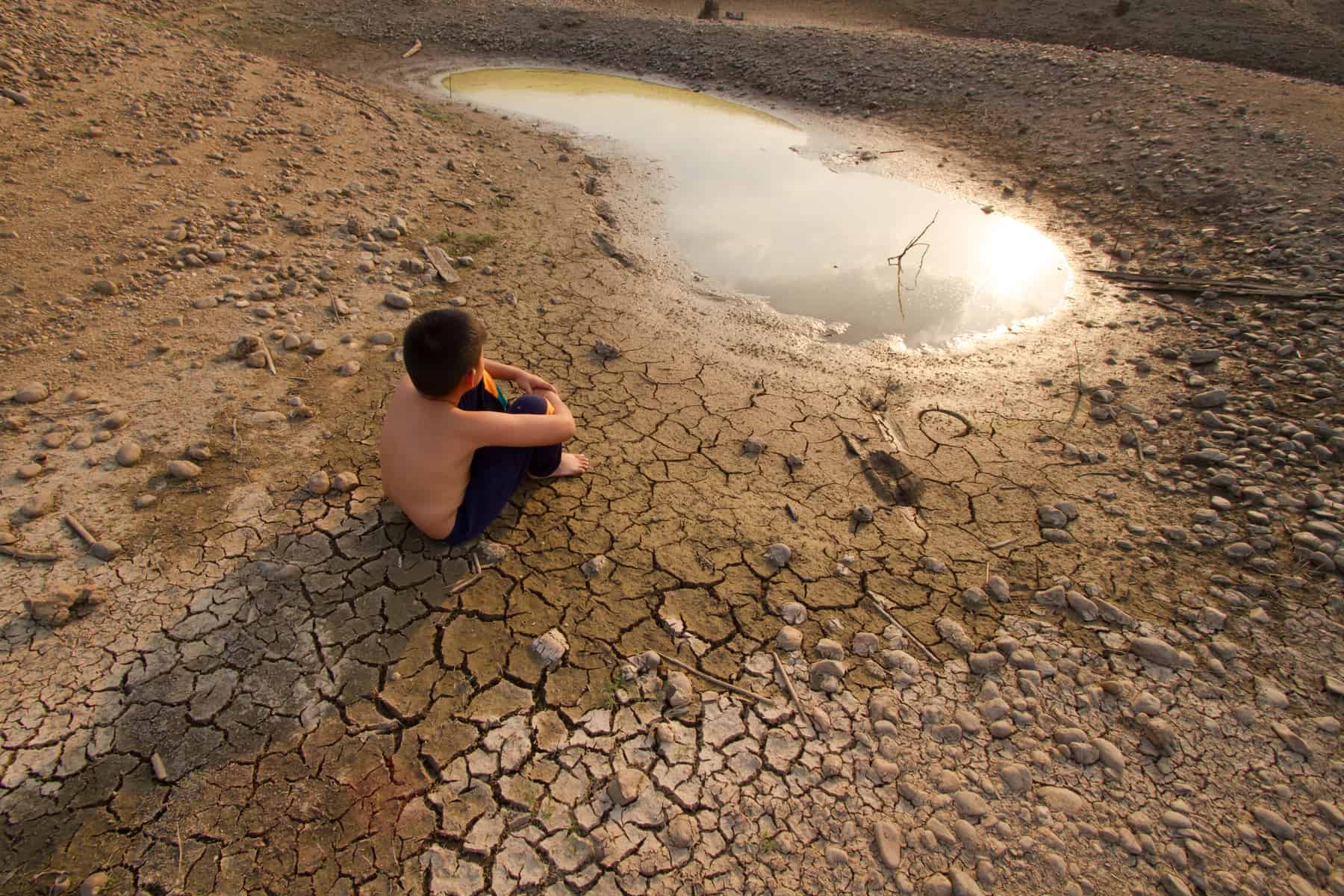
My biggest fear is that we will—or maybe already have—become parochial in our approach to this global challenge. That by choosing not to act in time or at the scale needed, we have condemned some of the poorest communities in the world—the already marginalized and vulnerable—to pay for the sins of our climatic excess. The fear used to be that those who have contributed the least to the problem will end up facing the worst climatic impacts. That, unfortunately, is now the reality.
What message would you like to give to the current generation of YSSPers?
Be bold in the questions you ask and the answers you seek. Never allow yourself—or anyone else—to rein in your intellectual ambition. Now is the time to think big. Because the challenges we face are gigantic.
Note: This article gives the views of the interviewee, and not the position of the Nexus blog, nor of the International Institute for Applied Systems Analysis.
Jul 15, 2016 | Alumni, Climate, Climate Change, Young Scientists
César Terrer, participant in the IIASA 2016 Young Scientists Summer Program, and PhD student at Imperial College London, recently made a groundbreaking contribution to the way scientists think about climate change and the CO2 fertilization effect. In this interview he discusses his research, his first publication in Science, and his summer project at IIASA.
Conducted and edited by Anneke Brand, IIASA science communication intern 2016.

César Terrer ©Vilma Sandström
How did your scientific career evolve into climate change and ecosystem ecology?
I studied environmental science in Spain and then I went to Australia, where I started working on free-air CO2 enrichment, or FACE experiments. These are very fancy experiments where you fumigate a forest with CO2 to see if the trees grow faster. In 2014 I moved to London for my PhD project. There, instead of focusing on one single FACE experiment, I collected data from all of them. This allowed me to make general conclusions on a global scale rather than a single forest.
You recently published a paper in Science magazine. Could you summarize the main findings?
We found that we can predict how much CO2 plants transfer into growth through the CO2 fertilization effect, based on two variables—nitrogen availability and the type of mycorrhizal, or fungal, association that the plants have. The impact of the type of mycorrhizae has never been tested on a global scale—and we found that it is huge. I think it’s fascinating that such tiny organisms play such a big role at a global scale on something as important as the terrestrial capacity of CO2 uptake.
How did you come up with the idea? One random day in the shower?
Long story short, researchers used to think that plants will grow faster, and take up a lot of the CO2 we emit. They assumed this in most of their models as well. But plants need other elements to grow besides CO2. In particular, they need nitrogen. So scientists started to question whether the modeled predictions overestimated the CO2 fertilization effect, because the models did not consider nitrogen limitation. To find out, I analyzed all the FACE experiments and indeed I saw that in general plants were not able to grow faster under elevated CO2 and nitrogen limitation. However, in some cases plants were able to take advantage of elevated CO2 even under nitrogen limitation. I grouped together the experiments where plants could grow under nitrogen limitation and after a lot of reading I saw what they had in common: the type of fungi! It turned out that one type of mycorrhizae is really good at transferring large quantities of nitrogen to the plant and the other type is not.
How did that feel?
Awesome! When I saw the graph, I knew: this is going to be important. Of course, after this, my coauthors helped me to polish the story. Without them, the conclusions would not be as robust and clear.
So how does this process work? Where do the fungi get the nitrogen from?
Particular soils might have a lot of nitrogen, but the amount available for plants to absorb might be low. Also, plants have to compete with non-fungal microorganisms for nitrogen. So if there is not much there, the microorganisms take it all. It’s called immobilization. Instead of mineralizing nitrogen, they immobilize it so that plants cannot take it up, at least not in the short term. Some types of fungi are much more efficient in accessing nitrogen, and associated with roots they allow plants to overcome limitations.
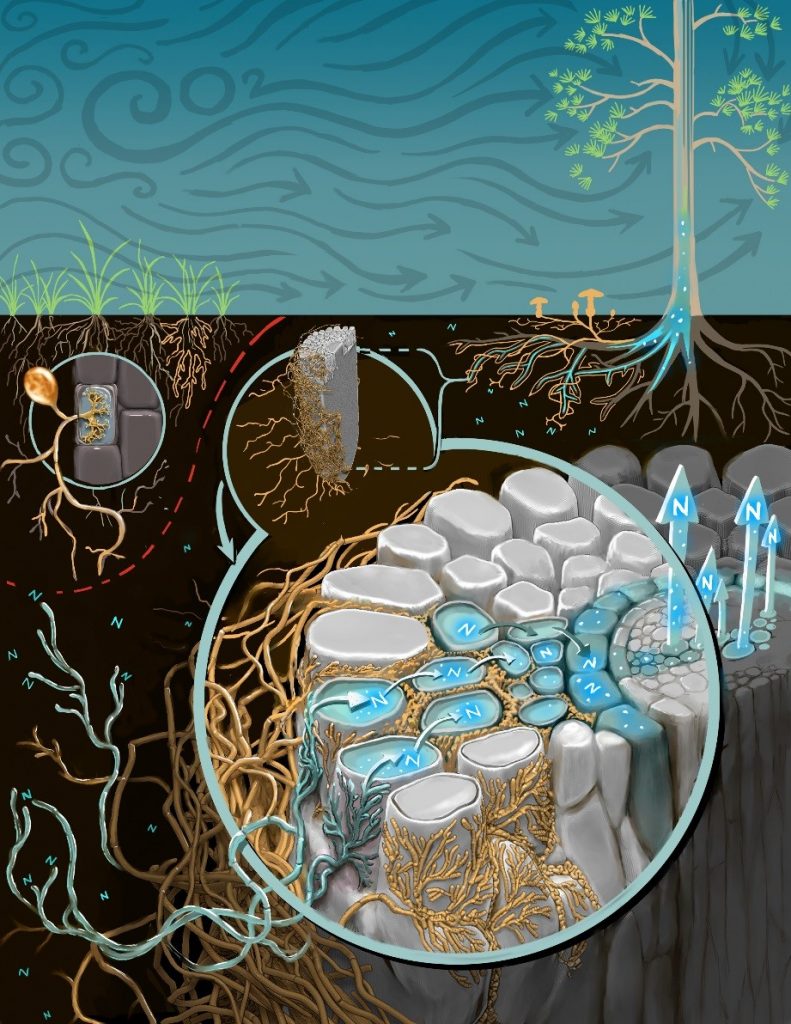
Nitrogen mobilization abilities of different types of fungi. Growth of plants associated with fungi not beneficial for nitrogen uptake (illustrated as grass roots on the left) could be limited by low nitrogen availability in soil. Other plants have the advantage of increased nitrogen uptake due to their beneficial association with certain types of fungi (illustrated as yellow mushrooms connected to the roots of the tree on the right). ©Victor O. Leshyk.
What is the impact of your findings?
Plants currently take up 25-30% of the CO2 we emit, but the question is whether they will be able to continue to do so in the long term. Our findings bring good and bad news. On the one hand, the CO2 fertilization effect will not be limited entirely by nitrogen, because some of the plants will be able to overcome nitrogen limitation through their root fungi. But on the other hand, some plant species will not be able to overcome nitrogen limitation.
There was a big debate about this. One group of scientists believed that plants will continue to take up CO2 and the other group said that plants will be limited by nitrogen availability. These were two very contrasting hypotheses. We discovered that neither of the hypotheses was completely right, but both were partly true, depending on the type of fungi. Our results could bring closure to this debate. We can now make more accurate predictions about global warming.
What will you do at IIASA and how will you link it to your PhD?
I want to upscale and quantify how much carbon plants will take up in the future. If we are to predict the capacity of plants to absorb CO2, we need to quantify mycorrhizal distribution and nitrogen availability on a global scale. We are updating mycorrhizal distribution maps according to distribution of plant species. We know for instance that pines are associated with ectomycorrhizal fungi and always will be. To quantify nitrogen availability we use maps of different soil parameters that are available on a rough global scale.

© Adam Edwards | Dreamstime.com
About César Terrer
Prior to his PhD, Terrer studied at the University of Murcia in Spain and the University of Western Sydney in Australia.
Currently he is a member of the Department of Life Sciences at Imperial College London, UK. For this study he collaborated with researchers from the University of Antwerp, Northern Arizona University, Indiana University and Macquarie University.
In the IIASA Young Scientists Summer Program, Terrer works together with Oskar Franklin from the Ecosystem Services and Management Program and Christina Kaiser from the Evolution and Ecology Program.
Further reading
Note: This article gives the views of the interviewee, and not the position of the Nexus blog, nor of the International Institute for Applied Systems Analysis.
Aug 13, 2015 | Energy & Climate
By Sabine Fuss, Mercator Research Institute on Global Commons and Climate Change (MCC) and IIASA Ecosystems Services and Management Program

The Sleipner CCS plant in Norway was the world’s first commercial CO2 storage facility. Photo: Kjetil Alsvik/Statoil
Current strategies for limiting climate change to no more than 2°C above pre-industrial levels are centered around a shift towards less carbon-intensive technology, increases in energy efficiency, and changes in management and behavior.
This won’t be enough.
Global carbon dioxide concentrations have exceeded the benchmark of 400ppm, and it is clear that we’re headed for an overshoot. This means that to have a chance of stabilizing climate change below 2°C, we will actually need to extract greenhouse gases from the atmosphere, thus achieving what we call “negative emissions.” This is even more evident when we look at continued population growth, our dependence on existing infrastructure in the near future, and rising living standards in many emerging regions.
In a session on negative emissions at this year’s CFCC conference in Paris jointly organized by members of the Global Carbon Project at IIASA, MCC and CSIRO, and CO2-GEONET, a group of leading international researchers discussed the need for negative emissions and the implications of large-scale removal of CO2 from the atmosphere, and took a closer look at the outstanding questions and uncertainties on the topic.

Bioenergy with Carbon Capture and Storage (BECCS), and afforestation are two possibilities that could contribute to negative emissions, removing greenhouse gases from the atmosphere. © zlikovec |Dollar Photo Club
A wide range of possibilities – but many open questions
The IPCC’s AR5 scenarios show that negative emissions could be achieved by combining carbon-neutral Bioenergy with Carbon dioxide Capture and Storage (BECCS), but also through afforestation. Most of the ambitious climate stabilization pathways show that we would need BECCS by the middle of the century, even though the removed emissions would not outweigh the remaining positive emissions at that point, that is, we would not yet see net negative emissions.
More precisely, the most recent scenarios of Integrated Assessment Models (IAMs) show that to achieve the 2°C limit, negative emissions of up to 13.2 GtCO2-eq./yr in 2100 are needed. This could be reached by BECCS, which might run into problems as competing for land with other demands, or a technology known as Direct Air Capture, which is more energy-intensive. Enhanced Weathering and afforestation might also deliver negative emissions, though of a smaller magnitude. However, all the presented negative emission technologies have their limits and none is a silver bullet. Clearly, there are more cards in the deck than just BECCS and we will have to aim for a portfolio respecting limits and trade-offs with other policy goals, but also opportunities and synergies.
One glaring clear point: negative emissions cannot be used to continue “business as usual” and then remove the bulk of the emissions mid-century. The required carbon flows would simply be too large. At the same time, such a high-emissions world would bring with it major environmental feedbacks, such as ocean acidification. Thus, negative emissions have to be understood as just one element of a mitigation portfolio complementing drastic GHG emission reductions in the near term.
While the large-scale use of biomass and its impacts have been at the center of bioenergy discussions for a while, CCS will also need to be scaled up to massive amounts of up to 25 GtCO2 per year by 2100. However, geology experts at the meeting were optimistic with respect to the storage potentials for these large amounts. The only challenge would be to find enough viable storage sites with assured capacity.
Other challenges include the need to investigate negative emission options that are not yet included in the AR5 scenarios, such as Enhanced Weathering, Direct Air Capture, and a method to improve CCS and BECCS with geothermal energy. How much the combined potential of these negative emissions options will indeed reduce temperatures also depends on the response of the climate system. However, two modelling teams presented new insights on reaction to overshoot, and negative emissions physically needed to keep global warming below 2°C.
While negative emissions are needed at large scale, many questions remain, which will need to be addressed very soon in order for scenarios meet reality. Communication must improve between scientists, politicians, practitioners, but also media and the public. Existing misunderstandings, for example, that negative emissions are just an excuse to continue on a business as usual pathway, or that negative emissions carry the same risks as geo-engineering, need to be resolved.
Read the full session report (PDF)
Sabine Fuss is leading the working group “Sustainable resource management and global change” at the Mercator Research Institute on Global Commons and Climate Change (MCC) in Berlin and holds a guest affiliation with IIASA’s ESM program. She is co-leading (with D. v. Vuuren) the research initiative “MAnaging Global Negative Emission Technologies (MaGNET)” hosted at the GCP Tsukuba Office
Note: This article gives the views of the author, and not the position of the Nexus blog, nor of the International Institute for Applied Systems Analysis.
48.055043416.3526776
Jun 23, 2015 | Energy & Climate, Science and Policy
By Hannes Böttcher, Senior Researcher, Öko-Institut, previously in IIASA’s Ecosystem Services and Management Program
In or out? Debit or credit? The role of the land use sector in the EU climate policy still needs to be defined
The EU has a target to reduce greenhouse gas emissions by at least 40% by 2030. This is an economy-wide target and therefore includes the land use sector, which includes land use, land use change and forestry. The EU is currently in the process of deciding how to integrate land use into this target. This is not an easy task, as we show in a new study.

Land use includes activities, such as logging, that can release greenhouse gases into the atmosphere. But the sector also includes other processes that can remove greenhouse gases from the atmosphere. Accounting for these processes is a complicated task. © Souvenirpixels | Dreamstime.com
The land use sector has several particularities that make it different from other sectors already included in the target, such as energy, industrial processes, waste, and agriculture. The most specific particularity is that the sector includes activities that cause emissions but also can lead to carbon being removed from that atmosphere, and taken up and stored in vegetation and soil. However, this removal is not permanent. Harvesting trees, and burning wood releases the carbon much more quickly than it was stored. Another particularity is that not all emissions and removals are directly caused by humans. This is especially true for removals from forest management.
In the past, the EU reported that uptake and storing of carbon through land use activities was higher than emissions from this sector. The European land use sector thus acted as a relatively stable net sink of emissions at around -300 to -350 Megatons (Mt) CO2 per year. But this might change in the near future: projections show the net sink declining to only 279 Mt CO2 in 2030.
Adding up carbon credits and debits
The emissions and removals that are actually occurring in the atmosphere are not exactly those that are currently accounted for under the Kyoto Protocol. Rather complicated rules exist that define what can be counted as credits and debits. Depending on how these rules develop, the EU sink may be accounted for to a large degree as a credit, or it could turn into a debit because the sink is getting smaller compared to the past. It is not likely that the entire sink will be turned into credits. Especially for the management of existing forests, which contributes a lot to the net sink, negotiators of the Kyoto Protocol have developed special accounting rules for the time before 2020. Under these rules, carbon credits only count if measured against a baseline.
The rules for the time after 2020 have not yet been agreed, however, as the Kyoto Protocol ends in 2020. In order to assess the impact of including the land use sector in the EU target in our new study, we had to make different assumptions, for example about how much wood we will harvest, the development of emissions and removals, and what the baseline for forest management should be. We then applied the existing Kyoto rules and alternative rules and assessed their impact on the level of ambition required to meet the EU’s target. It quickly became obvious: the assumptions we make and the rules we apply have very large implications for the 2030 Climate and Energy Framework.
One option of including land use discussed by the Commission is to take agriculture emissions out of the currently existing framework of the so-called ESD (an already existing mechanism to distribute mitigation efforts among EU Member States for specific sectors such as transport, buildings, waste and agriculture) and merge it with land use activities in a separate pillar. In our study we estimated the net credits that the land use sector could potentially generate, and found these credits could be as high as the entire emission reduction effort needed in agriculture. This would mean that in agriculture no reductions would be needed if the credits from land use were exchangeable between the sectors.
The impact on t he target of 40% emissions reductions can be more than 4 percentage points if land use is included and the rules are not changed. This means that the original 40% target without land use would be reduced to an only 35% target. Other sectors would have to reduce their emissions less because land use seems to do part of the job. The target as a whole would thus become much less ambitious than it currently is. But this does not need to be the case. If accounting rules are changed in a way to account for the fact that the sink is getting smaller and smaller, land use would create debits. Including debits in the target would make it a 41% target instead and increase the overall level of ambition. This would be bad for the atmosphere because effectively emissions would not be reduced as much as needed.
It thus all depends on assumptions and rules. Before the rules are announced, the contribution of the land use sector cannot be quantified. Given this, we argue that the best option would be to keep land use separate from other sectors, give it separate target and design accounting rules that set incentives to increase the sink.
Reference
Böttcher H, Graichen J. 2015. Impacts on the EU 2030 climate target of inlcuding LULUCF in the climate and energy policy framework. Report prepared for Fern and IFOAM. Oeko-Institut.
Note: This article gives the views of the author, and not the position of the Nexus blog, nor of the International Institute for Applied Systems Analysis.
Jan 19, 2015 | Energy & Climate
By Armon Rezai, Vienna University of Economics and Business Administration and IIASA,
and Rick van der Ploeg, University of Oxford, U.K., University Amsterdam and CEPR
The biggest externality on the planet is the failure of markets to price carbon emissions appropriately (Stern, 2007). This leads to excessive fossil fuel use which induces global warming and all the economic costs that go with it. Governments should cease the moment of plummeting oil prices and set a price of carbon equal to the optimal social cost of carbon (SCC), where the SCC is the present discounted value of all future production losses from the global warming induced by emitting one extra ton of carbon (e.g., Foley et al., 2013; Nordhaus, 2014). Our calculations suggest a price of $15 per ton of emitted CO2 or 13 cents per gallon gasoline. This price can be either implemented with a global tax on carbon emissions or with competitive markets for tradable emission rights and, in the absence of second-best issues, must be the same throughout the globe.
The most prominent integrated assessment model of climate and the economy is DICE (Nordhaus, 2008; 2014). Such models can be used to calculate the optimal level and time path for the price of carbon. Alas, most people including policy makers and economists view these integrated assessment models as a “black box” and consequently the resulting prescriptions for the carbon price are hard to understand and communicate to policymakers.

© Cta88 | Dreamstime.com
New rule for the global carbon price
This is why we propose a simple rule for the global carbon price, which can be calculated on the back of the envelope and approximates the correct optimal carbon price very accurately. Furthermore, this rule is robust, transparent, and easy to understand and implement. The rule depends on geophysical factors, such as dissipation rates of atmospheric carbon into oceanic sinks, and economic parameters, such as the long-run growth rate of productivity and the societal rates of time impatience and intergenerational inequality aversion. Our rule is based on the following premises.
- First, the carbon cycle dynamics are much more sluggish than the process of growth convergence. This allows us to base our calculations on trend growth rates.
- Second, a fifth of carbon emission stays permanently in the atmosphere and of the remainder 60 percent is absorbed by the oceans and the earth’s surface within a year and the rest has a half-time of three hundred years. After 3 decades half of carbon has left the atmosphere. Emitting one ton of carbon thus implies that is left in the atmosphere after t years.
- Third, marginal climate damages are roughly 2.38 percent of world GDP per trillion tons of extra carbon in the atmosphere. These figures come from Golosov et al. (2014) and are based on DICE. It assumes that doubling the stock of atmospheric carbon yields a rise in global mean temperature of 3 degrees Celsius. Hence, the within-period damage of one ton of carbon after t years is
- Fourth, the SCC is the discounted sum of all future within-period damages. The interest rate to discount these damages r follows from the Keyes-Ramsey rule as the rate of time impatience r plus the coefficient of relative intergenerational inequality aversion (IIA) times the per-capita growth rate in living standards g. Growth in living standards thus leads to wealthier future generations that require a higher interest rate, especially if IIA is large, because current generations are then less prepared to sacrifice current consumption.
- Fifth, it takes a long time to warm up the earth. We suppose that the average lag between global mean temperature and the stock of atmospheric carbon is 40 years.
We thus get the following back-of-the-envelope rule for the optimal SCC and price of carbon:

where r = ρ+ (IIA-1)x g. Here the term in the first set of round brackets is the present discounted value of all future within-period damages resulting from emitting one ton of carbon and the term in the second set of round brackets is the attenuation in the SCC due to the lag between the change in temperature and the change in the stock of atmospheric carbon.
Policy insights from the new rule
This rule gives the following policy insights:
- The global price of carbon is high if welfare of future generations is not discounted much.
- Higher growth in living standards g boosts the interest rate and thus depresses the optimal global carbon price if IIA > 1. As future generations are better off, current generations are less prepared to make sacrifices to combat global warming. However, with IIA < 1, growth in living standards boosts the price of carbon.
- Higher IIA implies that current generations are less prepared to temper future climate damages if there is growth in living standards and thus the optimal global price of carbon is lower.
- The lag between temperature and atmospheric carbon and decay of atmospheric carbon depresses the price of carbon (the term in the second pair of brackets).
- The optimal price of carbon rises in proportion with world GDP which in 2014 totalled 76 trillion USD.
The rule is easy to extend to allow for marginal damages reacting less than proportionally to world GDP (Rezai and van der Ploeg, 2014). For example, additive instead of multiplicative damages resulting from global warming gives a lower initial price of carbon, especially if economic growth is high, and a completely flat time path for the price of carbon. In general, the lower elasticity of climate damages with respect to GDP, the flatter the time path of the carbon price.
Calculating the optimal price of carbon following the new rule
Our benchmark set of parameters for our rule is to suppose trend growth in living standards of 2 percent per annum and a degree of intergenerational aversion of 2, and to not discount the welfare of future generations at all (g = 2%, IIA = 2, r = 0). This gives an optimal price of carbon of $55 per ton of emitted carbon, $15 per ton of emitted CO2, or 13 cents per gallon gasoline, which subsequently rises in line with world GDP at a rate of 2 percent per annum.
Leaving ethical issues aside, our rule shows that discounting the welfare of future generations at 2 percent per annum (keeping g = 2% and IIA = 2) implies that the optimal global carbon price falls to $20 per ton of emitted carbon, $5.5 per ton of emitted CO2, or 5 cents per gallon gasoline.
If society were to be more concerned with intergenerational inequality aversion and uses a higher IIA of 4 (keeping g = 2%, r = 0), current generations should sacrifice less current consumption to improve climate decades and centuries ahead. This is why our rule then indicates that the initial optimal carbon price falls to $10 per ton of carbon. Taking a lower IIA of one and a discount rate of 1.5% per annum as in Golosov et al. (2014) pushes up the initial price of carbon to $81 per ton emitted carbon.
A more pessimistic forecast of growth in living standards of 1 instead of 2 percent per annum (keeping IIA = 2, r = 0) boosts the initial price of carbon to $132 per ton of carbon, which subsequently grows at the rate of 1 percent per annum. To illustrate how accurate our back-of-the-envelope rule is, we road-test it in a sophisticated integrated assessment model of growth, savings, investment and climate change with endogenous transitions between fossil fuel and renewable energy and forward-looking dynamics associated with scarce fossil fuel (for details see Rezai and van der Ploeg, 2014). The figure below shows that our rule approximates optimal policy very well.

The table below also confirms that our rule also predicts the optimal timing of energy transitions and the optimal amount of fossil fuel to be left unexploited in the earth very accurately. Business as usual leads to unacceptable degrees of global warming (4 degrees Celsius), since much more carbon is burnt (1640 Giga tons of carbon) than in the first best (955 GtC) or under our simple rule (960 GtC). Our rule also accurately predicts by how much the transition to the carbon-free era is brought forward (by about 18 years). No wonder our rule yields almost the same welfare gain as the first best while business as usual leads to significant welfare losses (3% of world GDP).
Transition times and carbon budget
|
|
Fossil fuel Only |
Renewable Only |
Carbon used |
maximum temperature |
Welfare loss |
| IIA=2 |
First best |
2010-2060 |
2061 – |
955 GtC |
3.1 °C |
0% |
| Business as usual |
2010-2078 |
2079 – |
1640 GtC |
4.0 °C |
– 3% |
| Simple rule |
2010-2061 |
2062 – |
960 GtC |
3.1 °C |
– 0.001% |
Recent findings in the IPCC’s fifth assessment report support our findings. While it is not possible to translate their estimates of the social cost of carbon into our model in a straight-forward manner, scenarios with similar levels of global warming yield similar time profiles for the price of carbon.
Our rule for the global price of carbon is easy to extend for growth damages of global warming (Dell et al., 2012). This pushes up the carbon tax and brings forward the carbon-free era to 2044, curbs the total carbon budget (to 452 GtC) and the maximum temperature (to 2.3 degrees Celsius). Allowing for prudence in face of growth uncertainty also induces a marginally more ambitious climate policy, but rather less so. On the other hand, additive damages leads to a laxer climate policy with a much bigger carbon budget (1600 GtC) and abandoning fossil fuel much later (2077).
In sum, our back-of-the-envelope rule for the optimal global price of carbon and gives an accurate prediction of the optimal carbon tax. It highlights the importance of economic primitives, such as the trend growth rate of GDP, for climate policy. We hope that as the rule is easy to understand and communicate, it might also be easier to implement.
References
Dell, Melissa, Jones, B. and B. Olken (2012). Temperature shocks and economic growth: Evidence from the last half century, American Economic Journal: Macroeconomics 4, 66-95.
Foley, Duncan, Rezai, A. and L. Taylor (2013). The social cost of carbon emissions. Economics Letters 121, 90-97.
Golosov, M., J. Hassler, P. Krusell and (2014). Optimal taxes on fossil fuel in general equilibrium, Econometrica, 82, 1, 41-88.
Nordhaus, William (2008). A Question of Balance: Economic Models of Climate Change, Yale University Press, New Haven, Connecticut.
Nordhaus, William (2014). Estimates of the social cost of carbon: concepts and results from the DICE-2013R model and alternative approaches, Journal of the Association of Environmental and Resource Economists, 1, 273-312.
Rezai, Armon and Frederick van der Ploeg (2014). Intergenerational Inequality Aversion, Growth and the Role of Damages: Occam’s Rule for the Global Carbon Tax, Discussion Paper 10292, CEPR, London.
Stern, Nicholas (2007). The Economics of Climate Change: The Stern Review, Cambridge University Press, Cambridge.
Note: This article gives the views of the authors, and not the position of the Nexus blog, nor of the International Institute for Applied Systems Analysis.


You must be logged in to post a comment.